Temporal evolutions of three growth rates of M, V, and nominal GDP

In a previous article, "A three-piece set for understanding the money circulation", we introduced two formulations of money circulation, M=G+I and V=1/(1-β). In another previous article, "A relationship between nominal GDP growth rate and  government spending growth rate", we introduced a relationship between the above two growth rates. In this article, we show temporal evolutions of three growth rates on M, V, and nominal GDP (Y).

Growth rate of nominal GDP (y-axis) and growth rate of M=G+I (x-axis).

This plot shows growth rates of M=G+I and nominal GDP. These growth rates are directly proportional with some variance. Under the flow of money circulation, magnitude of M=G+I determines magnitude of nominal GDP. This is a causal relationship.

From this result, we can conclude that the low growth rate of Japanese GDP in recent years comes from the low growth rate of M=G+I.

Contents.

• Growth rates of M=G+I and V=1/(1-β).
• Nominal GDP Growth Rates of Japan and USA.
• Characteristics of the growth rate of V.

1. Growth rates of M=G+I and V=1/(1-β)

In this article, we introduce temporal evolutions of growth rates of M, V, and nominal GDP. These growth rates have the following relationships.

• dY/Y = dM/M + dV/V

This relation is derived from Y=MV, Fisher's equation of exchange. Here dY, dM, and dV are the small variations for each variable. We obtain this relation of the growth rates via two step. First is to expand an equation, Y+dY = (M+dM)(V+dV). Second is to omit a quadratic term, dMdV. If dY, dM, and dV are enough small, we can omit this quadratic term.

For these growth rates, we substitute actual values as follows,

• dY/Y = (Y2-Y1)/Y1.

Here, Y1 is the value of the previous year., and Y2 is the value of the current year. From this definition, we can obtain a growth rate compared to the previous year.

The data we used are published by the governments of Japan and USA. In the following, we show plots for the United States, Japan from 1956 to 1998, and Japan from 1995 to 2019. Two periods for Japan are because of different definitions of nominal GDP.

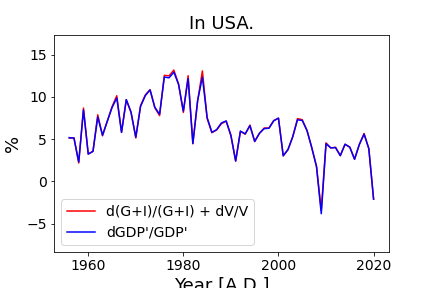
In the following plots, we use GDP', which is GDP minus net exports (EX-IM). This is because net exports are not related to the money circulation and Y=C+G+I.

2. Nominal GDP growth rates in Japan and USA

The following plots are on USA.

In the first plot, the blue line shows dY/Y. And the red line shows the sum of dM/M and dV/V. In the second plot, the blue line indicates dY/Y, the redline indicates dM/M, and the black line indicates dV/V.

As is shown in the second plot, dY/Y and dM/M shows good correlation. And dV/V is roughly in the range of about ±2%. In other words, dY/Y and dM/M are well correlated with a variance of around ±2%.

This relation between dY/Y, dM/M and dV/V is because temporal variation of the average propensity to consume (β) is smaller than that of M=G+I, in the data set.

Prior to the 1960s, dV/V was sometimes smaller than -5%. After that, dV/V was in the range of a few percentage. Therefore, after 1970, dY/Y and dM/M are well correlated.

The large negative values of dV/V before the 1960s means decrease of V. This also means decrease of the average propensity to consume. This change indicates a change of the economic structure in Japan. For example, day laborers had decreased, and many people had started to save and obtain a stable life.

Since 1995, dY/Y, dM/M, and dV/V shows comparable values within ±5%. An exception is Lehman Brothers collapsed in 2009.

Again, we show the scatter plot between growth rates of M=G+I and nominal GDP.

As is shown in the above scatter plot, from the money circulation, the growth rate of G+I controls the growth rate of nominal GDP. From this realization, several important things are shed light on.

First is the low growth of Japan's nominal GDP in recent years. Some Japanese people think that this low growth rate is owing to laziness of Japanese people. However, this low growth rate is owing to the low growth rate of G+I, and is not owing to laziness of Japanese people.

Second is that an innovative product in individual markets has no relation with growth of nominal GDP. When science and technology increase the total number of goods and services (e.g. railways, and IT technology), G+I and nominal GDP increase.

Third is that all previous works to predict nominal GDP growth in macroeconomics come to naught. This is because present macroeconomics is based mainly on equilibrium of supply and demand, and not on money circulation.

3. Characteristics of the growth rate of V

Readers may have two questions on dV/V in the above plots. One is why dV/V is around the range of ±2%. Another is why increase and decrease of dV/V takes the opposite direction to those of dY/Y and dM/M. For example, when growth rates of dY/Y and dM/M increase, growth rate of dV/V decrease. And vice versa.

On "2%," we must consider it quantitatively. It is going to be long, so I'd like to summarize my discussion in another article or e-book. We showed a scatter plot of dM/M and dV/V in section 4.2 of the e-book "Macroflow Economics 3 Quantitative Analysis of the Money Circulation". The following is that scatter plot. (Note that this derivation for M and V is slightly different from M=G+I and V=1/(1-β).)

Clearly, we can see a certain gradient in this plot. For discussion on this gradient, we need some ideas on V. Money circulation velocity V is not precisely discussed in the modern macroeconomics.

Link page: Contents for money circulation